
CERF Blog
I have written several essays lately on various aspects of what I call the Sustainable Financial Plan (SFP). My colleague at CLU, Bill Watkins, suggests that I produce a simplified version of these essays that is targeted for young people (I think this is Bill’s nice way of saying that the original essays were indecipherable).
So, this essay contains the key elements of the Simplified Sustainable Financial Plan (SSFP).
The basic idea is to put together a plan that has no or very little chance of failure, where failure means to run your wealth down to zero.
Step 1: Predict future earnings
The first step is to recognize the importance of what economists call “human capital.” This is the present value of your future (after-tax) earnings stream. What does this mean? Your earnings “stream” is the series of annual incomes, from now until retirement. Naturally, since this earnings stream lies in the future, we can’t know exactly what it is today. But, there is a lot of historical data on incomes as a function of occupation, education and experience. Based on data in the Federal Reserves’ Survey of Consumer Finances, shown below are income age profiles (that is, income as a function of age) for high school and college graduates.
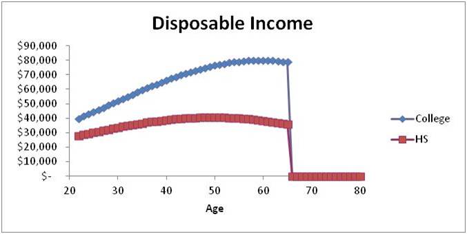
These profiles are for the median individual in each group. This means fifty percent will have higher earnings and fifty percent will have lower earnings. Note that the median college graduate enjoys roughly a doubling of real income over his or her working career.
How can you come up with something like this for yourself? Well, you can use these median estimates. Or, you can do better by including additional data like your current wage, information on average wages in your chosen field, etc.
As you progress through your career, you will continually be compiling new data with which to modify your estimate.
Step 2: Estimate the after-tax real rate of return on investment
Suppose you have a portfolio of financial assets such as stocks and bonds. The rate of return on investment is the rate at which the portfolio will grow (over time, we hope, the average rate of return will be positive). Growth can come through increases in the price of the assets or through interest or dividend payments. For example, over the past hundred years or so the overall U.S. stock market has thrown off returns of approximately ten percent, before taxes and before adjusting for inflation. Adjusting for taxes and inflation, the real after-tax equity return has averaged about 7% over the long haul.
Estimating the future real return is a pretty complex undertaking. To simplify, let’s suppose there are two asset classes – stocks and bonds. Further, let’s suppose the expected real after-tax rate of return on stocks is 6% and on bonds is 0%. A fifty/fifty allocation between stocks and bonds will then have an expected return of 3%. Thus, let’s say that we believe 3% is a reasonably conservative estimate of the real after-tax rate of return.
Step 3: Calculate the value of human capital
The next step is to discount the future income stream by the 3% rate of return. That is, we find the present value of the future income. What does this mean? Suppose you have $10,000 today and you invest it at 3% for one year. One year later you will have $10,300. The “present value” today of $10,300 one year in the future is $10,000. If you apply this idea to your projected income each year in the future and then add up the present values, you have the present value of future income. This is what we call human capital (HC). The rationale for using the financial rate of return for the discount rate is simply that were we to have a portfolio of this size today, invested at 3% return, we could generate the series of future after-tax real incomes.
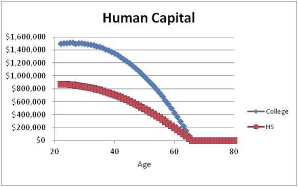
The chart shows the age profile of human capital for the median high school graduate and median college graduate. To see how we get this “age profile” suppose our college graduate is 22 years old. The first number on the chart is the present value of income from age 22 to retirement. The second number on the chart is the present value of income from age 23 to retirement, and so on.
Notice several features of the chart. First, the HC of the college graduate is more than 50% higher ($600,000 greater) than the HC of the high school graduate. This suggests a very significant return to graduating from college. Second, at some point the HC peaks out and begins to decline. This will necessarily occur as you approach retirement. However, it is likely that HC can be improved a lot early in your career. For one thing, you can increase HC by going to school. Or you can increase HC through experience on the job and career management. Almost surely, the most important element of your financial plan is how you manage your human capital.
The last point to note about this chart is simply that the value of human capital for young people is really big. For the median college grad it is over $1.4 million, and for the median high school grad it is more than $800,000.
Step 4: Calculate Wealth as the sum of Human Capital and Financial Capital
Total wealth is the sum of human capital and “financial capital” (FC) which is the value of assets less the value of debt. Financial capital is what most people refer to as net worth. For young people, wealth is primarily human capital. For people closer to or in retirement, human capital is small and the bulk of wealth is in the form of financial capital. The essence of the SSFP is that people should save out of current income enough so as to increase the value of FC to offset eventual declines in the value of HC.
The baby boom generation, on average, did not do this. Compare the human capital in the previous chart to the wealth of the median baby boomer nearing retirement. The Fed’s Survey of Consumer Finances suggests that median wealth for people aged 55-65 is only about $250,000. This means that kids today are quite a bit richer than their parents and grandparents! How can this be? The simple answer is that the typical baby boomer did not save enough throughout their lifetime.
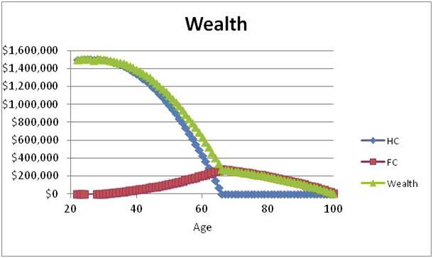
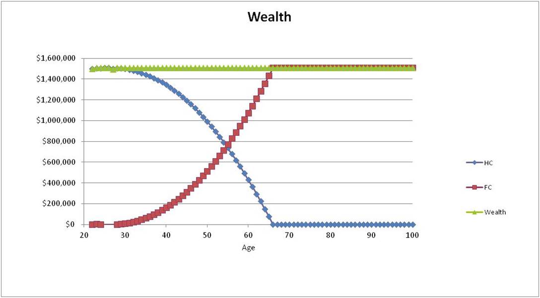
The chart shows human capital, financial capital and their sum, wealth, for the typical baby boomer. HC peaked out around $1.4 million (in today’s dollars) back when the boomer was around 30 years old and then began to decline. The boomer savings rate was positive but low and the accumulated FC at retirement for the typical boomer will not support the accustomed rate of consumption spending. That leaves basically two options for the boomer: reduce consumption in retirement or delay the date of retirement.
There are two factors that drive financial capital. The first is your savings rate and the second is your investment strategy.
Step 5: Calculate a consumption path that preserves wealth
By spending less than disposable income, and then managing your investment portfolio, you can build up financial capital. The major error made by many baby boomers is that they allowed total wealth to decline. They did this partly because “experts” advised them to do so. Many financial advisors recommend strategies that call for declining wealth. Economists sometimes argue that the objective of personal financial planning is to die broke. The reason for this is that if you don’t die broke then you have foregone potential consumption, and the goal of economic life is to maximize consumption.
I think this is an error. For one thing, you do not know when you are going to die, so allowing your wealth to decline risks becoming broke before you die. For another, there is a lot to be said for building and hanging onto financial wealth. This will give you lots of valuable options in your later years; options like assisting family members, supporting charities, or financing ventures. Also, by attempting to preserve your wealth you automatically build in financial cushions against unexpected shocks, which tend to occur a lot more frequently than most of us expect.
A simple consumption rule that preserves wealth is to set consumption equal to wealth multiplied by the estimated return from Step 2. Take the example of the median college grad mentioned earlier. This individual’s human capital is $1.4 million. Let’s suppose financial capital is zero. Using 3% as our estimate of return, we come up with $1.4M*3%=$42,000 as the sustainable consumption level.
If the college graduate adopts and sticks with this spending plan, he or she will accumulate FC in excess of $1 million by the time of retirement. That’s not $1 million in future deflated dollars; that is $1 million in current dollars.
Step 6: Always save something
It is possible, even likely for young people with rapidly growing incomes, that the sustainable consumption level is greater than current disposable income. In this event, it is advisable to lower your consumption level to 90% of disposable income. This allows you to take advantage of what Einstein is reputed to have said is the most powerful force in the universe – compounding. By starting to build a financial asset portfolio as early as possible you get this force working for you. If you borrow to finance consumption in excess of disposable income, you have the most powerful force in the universe working against you.
To summarize the argument so far, set consumption equal to the minimum of 3% of wealth or 90% of disposable income. This keeps wealth from falling as you age.
So far, we have used a steady 3% investment return, and spending of 3% of wealth. The next step is to recognize that actual investment return will fluctuate.
Step 7: Adjust the consumption rule so as to stabilize consumption against shocks to wealth
So far we have come up with a consumption rule that is sustainable. But it is not necessarily stable. Fluctuations in asset prices can push wealth around a lot, particularly for older people whose wealth is predominately in the form of financial capital.
We propose two modifications to the basic spending rule, one to address declines in wealth and the other to address increases in wealth. Suppose your wealth falls, how should you adjust your spending? According to the basic rule, if wealth falls 10% then your spending should fall 10%. But it is possible, even likely that poor investment returns will be followed some time in the future by better returns, at least that is true if you have been reasonably conservative in estimating the return and in managing your portfolio. To avoid unnecessary declines in spending in response to temporary declines in wealth, we propose the Retrenchment Rule.
The Retrenchment Rule (the name comes from the title of a book by financial economist Gordon Pye) provides guidance about when you have to adjust your spending downward, or “retrench.” To implement the rule you need to calculate the value of a fixed lifetime annuity that you could purchase with your current wealth, using a very conservative estimate of how long you might possibly live. Insurance tables suggest that the probability of anyone living past the age of 110 is near zero. So, I propose calculating the fixed annuity (FA) based on current wealth, a 3% return, and assumed mortality at age 110. A fixed annuity is a constant payment from now to a terminal date. If this fixed annuity is greater than last year’s spending level, then you do not need to retrench at all. But if the fixed annuity is less than last year’s spending, then you have retrench back to the amount of the fixed annuity.
In short, the Retrenchment Rule says that consumption this period is the minimum of consumption last period and the fixed annuity.
What about responding to increases in wealth? If wealth increases substantially, it would seem reasonable to consider ratcheting up spending. The Ratchet Rule tells us when to do this. To implement the Ratchet Rule you need to specify another discount rate, equal to or lower than the expected rate of return. I propose 1% for this, but you can use something a bit higher, like 2% or even 3%, if you like. My rationale for the 1% Ratchet Rule is that if you follow this rule, you have a good chance to join the 1% net worth club (the “1% club”), that is, you have a good chance to eventually enjoy financial wealth greater than all but 1% of households. Today, that means wealth of approximately $5 million. The effect of the 1% Ratchet Rule is that you do not increase your consumption until your initial wealth triples. If you follow this rule then the chance of eventually reaching the 1% club is fairly good, even starting with zero financial capital (of course, this is true only if just a small fraction of people adopt the strategy; if everyone does, then the threshold for the 1% club will be a lot higher than it is today).
The 1% Ratchet Rule says that you can increase your spending whenever wealth increases to the point that 1% of wealth is greater than the current consumption level. That is, the Rule says that consumption this period should be the maximum of consumption last period and 1% of current wealth.
Again, you don’t have to choose 1% for the Ratchet Rule. If you choose 3%, then you will be led to ratchet up spending whenever your wealth increases. The effect is to enable greater consumption, but sharply reduce the chance of reaching the 1% club.
Simulations
To prove that your plan is stable and sustainable, it is important to subject the plan to random shocks in investment returns. The 3% return that we have been using is simply an estimate of the average rate of return over time. The actual return each year will be different. This is why we proposed the Retrenchment and Ratchet Rules. To test how these rules work, we need to simulate actual returns.
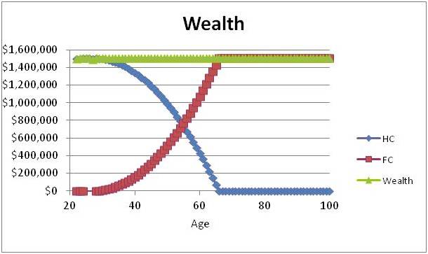
The chart below shows HC, FC and Wealth just as earlier charts have done. The difference is that growth in FC is driven by randomly simulated rates of return. We are assuming a 50/50 portfolio allocation between risky stocks and safe bonds. We can repeat this exercise hundreds or thousands of times and keep track of the performance of consumption spending and wealth. An important criterion for a sustainable plan is that the probability of running out of wealth is very close to zero. This can be tested by running 1,000 or more simulations and counting the number of times that wealth goes negative. The probability of plan failure is this number divided by 1,000.
Another interesting calculation is to count the number of scenarios in which wealth reaches $5 million. Dividing by 1,000 yields the probability of joining the 1% club.
Here is one simulation:
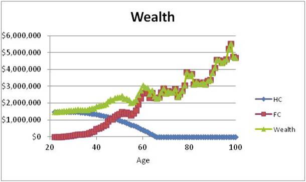
What is happening in the scenario shown here is that financial capital is increasing rapidly in retirement. This is because the series of randomly drawn annual returns is favorable. If you find yourself in a scenario like this you may want to increase consumption spending more rapidly than the 1% Ratchet Rule suggests. The beauty of the plan is that you are likely to have the opportunity to do so.
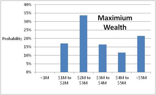
To implement the SSFP, we are creating a set of calculators at www.clucerf.org. These calculators allow the user to experiment with some of the key assumptions – like percent of financial capital allocated to equities, initial consumption level, retirement age, ratchet rule, etc. – and examine the consequences for the sustainability of the plan and stability of spending. A good way to do this is to collect the results of a large number of simulations. For example, using the parameter settings: 3% spending rate, 1% Ratchet Rule, 50/50 equity/bond mix, I get zero cases of plan failure (wealth reaches zero) in 1,000 simulations. And in just over 200 of the scenarios (20% of the time) wealth reaches the $5 million cutoff for the 1% net worth club.
Summary
The main features of the SSFP are first that you should measure and manage your human capital, and second you should adopt a spending plan that preserves wealth even as your human capital recedes.
